Mode (statistics)
In statistics, the mode is the value that occurs most frequently in a data set or a probability distribution.[1] In some fields, notably education, sample data are often called scores, and the sample mode is known as the modal score.[2]
Like the statistical mean and the median, the mode is a way of capturing important information about a random variable or a population in a single quantity. The mode is in general different from the mean and median, and may be very different for strongly skewed distributions.
The mode is not necessarily unique, since the same maximum frequency may be attained at different values. The most ambiguous case occurs in uniform distributions, wherein all values are equally likely.
Contents |
Mode of a probability distribution
The mode of a discrete probability distribution is the value x at which its probability mass function takes its maximum value. In other words, it is the value that is most likely to be sampled.
The mode of a continuous probability distribution is the value x at which its probability density function attains its maximum value, so, informally speaking, the mode is at the peak.
As noted above, the mode is not necessarily unique, since the probability mass function or probability density function may achieve its maximum value at several points x1, x2, etc.
The above definition tells us that only global maxima are modes. Slightly confusingly, when a probability density function has multiple local maxima it is common to refer to all of the local maxima as modes of the distribution. Such a continuous distribution is called multimodal (as opposed to unimodal).
In symmetric unimodal distributions, such as the normal (or Gaussian) distribution (the distribution whose density function, when graphed, gives the famous "bell curve"), the mean (if defined), median and mode all coincide. For samples, if it is known that they are drawn from a symmetric distribution, the sample mean can be used as an estimate of the population mode. The mode is if there is more than one number in the plot Example
1,2,2,3,4,5,5,6,5,1 The numbers that repeat are the mode. There can be more than one mode anytime
Mode of a sample
The mode of a data sample is the element that occurs most often in the collection. For example, the mode of the sample [1, 3, 6, 6, 6, 6, 7, 7, 12, 12, 17] is 6. Given the list of data [1, 1, 2, 4, 4] the mode is not unique - the dataset may be said to be bimodal, while a set with more than two modes may be described as multimodal.
For a sample from a continuous distribution, such as [0.935..., 1.211..., 2.430..., 3.668..., 3.874...], the concept is unusable in its raw form, since each value will occur precisely once. The usual practice is to discretize the data by assigning frequency values to intervals of equal distance, as for making a histogram, effectively replacing the values by the midpoints of the intervals they are assigned to. The mode is then the value where the histogram reaches its peak. For small or middle-sized samples the outcome of this procedure is sensitive to the choice of interval width if chosen too narrow or too wide; typically one should have a sizable fraction of the data concentrated in a relatively small number of intervals (5 to 10), while the fraction of the data falling outside these intervals is also sizable. An alternate approach is kernel density estimation, which essentially blurs point samples to produce a continuous estimate of the probability density function which can provide an estimate of the mode.
The following MATLAB code example computes the mode of a sample:
X = sort(x);
indices   =  find(diff([X; realmax]) > 0); % indices where repeated values change
[modeL,i] =  max (diff([0; indices]));     % longest persistence length of repeated values
mode      =  X(indices(i));
The algorithm requires as a first step to sort the sample in ascending order. It then computes the discrete derivative of the sorted list, and finds the indices where this derivative is positive. Next it computes the discrete derivative of this set of indices, locating the maximum of this derivative of indices, and finally evaluates the sorted sample at the point where that maximum occurs, which corresponds to the last member of the stretch of repeated values.
Comparison of mean, median and mode
| Type | Description | Example | Result |
|---|---|---|---|
| Arithmetic mean | Sum divided by number of values: 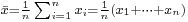 |
(1+2+2+3+4+7+9) / 7 | 4 |
| Median | Middle value separating the greater and lesser halves of a data set | 1, 2, 2, 3, 4, 7, 9 | 3 |
| Mode | Most frequent value in a data set | 1, 2, 2, 3, 4, 7, 9 | 2 |
When do these measures make sense?
Unlike mean and median, the concept of mode also makes sense for "nominal data" (i.e., not consisting of numerical values). For example, taking a sample of Korean family names, one might find that "Kim" occurs more often than any other name. Then "Kim" would be the mode of the sample. In any voting system where a plurality determines victory, a single modal value determines the victor, while a multi-modal outcome would require some tie-breaking procedure to take place.
Unlike median, the concept of mean makes sense for any random variable assuming values from a vector space, including the real numbers (a one-dimensional vector space) and the integers (which can be considered embedded in the reals). For example, a distribution of points in the plane will typically have a mean and a mode, but the concept of median does not apply. The median makes sense when there is a linear order on the possible values. Generalizations of the concept of median to higher-dimensional spaces are the geometric median and the centerpoint.
Uniqueness and definedness
For some probability distributions, the expected value may be infinite or undefined, but if defined, it is unique. The mean of a (finite) sample is always defined. The median is the value such that the fractions not exceeding it and not falling below it are both at least 1/2. It is not necessarily unique, but never infinite or totally undefined. For a data sample it is the "halfway" value when the list of values is ordered in increasing value, where usually for a list of even length the numerical average is taken of the two values closest to "halfway". Finally, as said before, the mode is not necessarily unique. Certain pathological distributions (for example, the Cantor distribution) have no defined mode at all. For a finite data sample, the mode is one (or more) of the values in the sample.
Properties
Assuming definedness, and for simplicity uniqueness, the following are some of the most interesting properties.
- All three measures have the following property: If the random variable (or each value from the sample) is subjected to the linear or affine transformation which replaces X by aX+b, so are the mean, median and mode.
- However, if there is an arbitrary monotonic transformation, only the median follows; for example, if X is replaced by exp(X), the median changes from m to exp(m) but the mean and mode won't.
- Except for extremely small samples, the mode is insensitive to "outliers" (such as occasional, rare, false experimental readings). The median is also very robust in the presence of outliers, while the mean is rather sensitive.
- In continuous unimodal distributions the median lies, as a rule of thumb, between the mean and the mode, about one third of the way going from mean to mode. In a formula, median ≈ (2 × mean + mode)/3. This rule, due to Karl Pearson, often applies to slightly non-symmetric distributions that resemble a normal distribution, but it is not always true and in general the three statistics can appear in any order.[3][4]
- For unimodal distributions, the mode is within
 standard deviations of the mean, and the root mean square deviation about the mode is between the standard deviation and twice the standard deviation.[5]
Example for a skewed distribution
An example of a skewed distribution is personal wealth: Few people are very rich, but among those some are extremely rich. However, many are rather poor.
A well-known class of distributions that can be arbitrarily skewed is given by the log-normal distribution. It is obtained by transforming a random variable X having a normal distribution into random variable Y = eX. Then the logarithm of random variable Y is normally distributed, hence the name.
Taking the mean μ of X to be 0, the median of Y will be 1, independent of the standard deviation σ of X. This is so because X has a symmetric distribution, so its median is also 0. The transformation from X to Y is monotonic, and so we find the median e0 = 1 for Y.
When X has standard deviation σ = 0.25, the distribution of Y is weakly skewed. Using formulas for the log-normal distribution, we find:
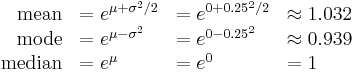
Indeed, the median is about one third on the way from mean to mode.
When X has a larger standard deviation, σ = 1, the distribution of Y is strongly skewed. Now
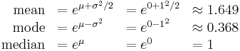
Here, Pearson's rule of thumb fails.
See also
- unimodal function
- summary statistics
- descriptive statistics
- central tendency
- arg max
- moment (mathematics)
References
- ^ Butler, Gregory (2010). "Mode". In Salkind, Neil. Encyclopedia of research design. Sage. pp. 140–142. ISBN 978-1-4129-6127-1.
- ^ The Math Dictionary - Didax Educational Resources
- ^ Relationship between the mean, median, mode, and standard deviation in a unimodal distribution
- ^ Paul T. von Hippel. Mean, Median, and Skew: Correcting a Textbook Rule. J. of Statistics Education 13:2 (2005)
- ^ Maximum distance between the mode and the mean of a unimodal distribution
External links
|
|||||||||||||||||||||||||||||||||||||||||||||||||||||||||||||||||||||||||||||||||||||||||||||||||||||||||||||||||||||||||||||||||||||||||||